- Published on

AI PROJECT-1.2 Download Dataset in JupyterLab or Jupyter Notebook
- Authors

- Name
- KAUSTUBH SHARMA
How to Download DataSet in Jupyter or JupyterLab?
STEP-0: (ONLY IF YOU ARE NOT USING SAGEMAKER NOTEBOOK INSTANCES, For SageMaker Notebook Instances user, proceed with Step-2)
- As we already using SageMaker Notebook Instance, So we don't need to install conda and other library package.
- But if we are working on a system which doesn't have Conda installed, you can install conda by Downloading from Here.
- Then to download datset, we require SHAP(SHapley Additive exPlanations) library, a popular tool for interpreting the output of machine learning models, which we can install using Conda using below code:
%conda install -c conda-forge shap
- If you're using JupyterLab, you have to manually refresh Jupyter kernel after the installation and updates have completed. Run the following IPython script to shut down the kernel (the kernel will restart automatically):
import IPython
IPython.Application.instance().kernel.do_shutdown(True)
STEP-1: Update Conda Version
- First, we will check current conda version using:
conda -V
- First we will update conda using below code:
conda update -n base -c conda-forge conda
- Then, again we will check current(updated) conda version using:
conda -V
STEP-2: Import SHAP Library
- First we need to import the SHAP(SHapley Additive exPlanations) library using below commands.
import shap #Import the SHAP library, a popular tool for interpreting the output of machine learning models.
STEP-3: Load DataSet
- Then, we have to load the Adult Census dataset (available here), also known as "Census Income" dataset to your notebook instance.
import shap # Import the SHAP library, a popular tool for interpreting the output of machine learning models.
X = shap.datasets.adult() #Load the Adult Census dataset using shap library
X  #Displays the value of X
Output:
(        Age  Workclass  Education-Num  Marital Status  Occupation  \
 0      39.0          7           13.0               4           1
 1      50.0          6           13.0               2           4
 2      38.0          4            9.0               0           6
 3      53.0          4            7.0               2           6
 4      28.0          4           13.0               2          10
 ...     ...        ...            ...             ...         ...
 32556  27.0          4           12.0               2          13
 32557  40.0          4            9.0               2           7
 32558  58.0          4            9.0               6           1
 32559  22.0          4            9.0               4           1
 32560  52.0          5            9.0               2           4

        Relationship  Race  Sex  Capital Gain  Capital Loss  Hours per week  \
 0                 0     4    1        2174.0           0.0            40.0
 1                 4     4    1           0.0           0.0            13.0
 2                 0     4    1           0.0           0.0            40.0
 3                 4     2    1           0.0           0.0            40.0
 4                 5     2    0           0.0           0.0            40.0
 ...             ...   ...  ...           ...           ...             ...
 32556             5     4    0           0.0           0.0            38.0
 32557             4     4    1           0.0           0.0            40.0
 32558             1     4    0           0.0           0.0            40.0
 32559             3     4    1           0.0           0.0            20.0
 32560             5     4    0       15024.0           0.0            40.0

        Country
 0           39
 1           39
 2           39
 3           39
 4            5
 ...        ...
 32556       39
 32557       39
 32558       39
 32559       39
 32560       39

 [32561 rows x 12 columns],
 array([False, False, False, ..., False, False,  True]))
- Jupyter Notebooks retain memory throughout the notebook.So, if I put X in the next cell like below, it will show the value of X.
X
Output:
(        Age  Workclass  Education-Num  Marital Status  Occupation  \
 0      39.0          7           13.0               4           1
 1      50.0          6           13.0               2           4
 2      38.0          4            9.0               0           6
 3      53.0          4            7.0               2           6
 4      28.0          4           13.0               2          10
 ...     ...        ...            ...             ...         ...
 32556  27.0          4           12.0               2          13
 32557  40.0          4            9.0               2           7
 32558  58.0          4            9.0               6           1
 32559  22.0          4            9.0               4           1
 32560  52.0          5            9.0               2           4

        Relationship  Race  Sex  Capital Gain  Capital Loss  Hours per week  \
 0                 0     4    1        2174.0           0.0            40.0
 1                 4     4    1           0.0           0.0            13.0
 2                 0     4    1           0.0           0.0            40.0
 3                 4     2    1           0.0           0.0            40.0
 4                 5     2    0           0.0           0.0            40.0
 ...             ...   ...  ...           ...           ...             ...
 32556             5     4    0           0.0           0.0            38.0
 32557             4     4    1           0.0           0.0            40.0
 32558             1     4    0           0.0           0.0            40.0
 32559             3     4    1           0.0           0.0            20.0
 32560             5     4    0       15024.0           0.0            40.0

        Country
 0           39
 1           39
 2           39
 3           39
 4            5
 ...        ...
 32556       39
 32557       39
 32558       39
 32559       39
 32560       39

 [32561 rows x 12 columns],
 array([False, False, False, ..., False, False,  True]))
STEP-4: Disaplaying Features and Labels
- We can see that X displays features(Age, Occupation, etc.) and labels(If Person's income exceeds $50K/yr, in form of 'True' or 'False').
- So, we need to seperate them using below code.
X, Y = shap.datasets.adult() #Load the Adult Census dataset using shap library, where features are assigned to X and labels to Y
X
Y
Output:
array([False, False, False, ..., False, False, True])
- As we can see from above code, only results of Y is displayed.
- But if you load individual value of X, it will show output.
X
Output:
Age	Workclass	Education-Num	Marital Status	Occupation	Relationship	Race	Sex	Capital Gain	Capital Loss	Hours per week	Country
0	39.0	7	13.0	4	1	0	4	1	2174.0	0.0	40.0	39
1	50.0	6	13.0	2	4	4	4	1	0.0	0.0	13.0	39
2	38.0	4	9.0	0	6	0	4	1	0.0	0.0	40.0	39
3	53.0	4	7.0	2	6	4	2	1	0.0	0.0	40.0	39
4	28.0	4	13.0	2	10	5	2	0	0.0	0.0	40.0	5
...	...	...	...	...	...	...	...	...	...	...	...	...
32556	27.0	4	12.0	2	13	5	4	0	0.0	0.0	38.0	39
32557	40.0	4	9.0	2	7	4	4	1	0.0	0.0	40.0	39
32558	58.0	4	9.0	6	1	1	4	0	0.0	0.0	40.0	39
32559	22.0	4	9.0	4	1	3	4	1	0.0	0.0	20.0	39
32560	52.0	5	9.0	2	4	5	4	0	15024.0	0.0	40.0	39
32561 rows × 12 columns
- And value of Y also will be displayed.
Y
Output:
array([False, False, False, ..., False, False, True])
- This tells us that Cells only displays result of last variable.
- And, to display results of results of variables other than last, we have to modify code as below:
display(X) #Displays the value of X
Y #Displays the value of Y
Output:
	Age	Workclass	Education-Num	Marital Status	Occupation	Relationship	Race	Sex	Capital Gain	Capital Loss	Hours per week	Country
0	39.0	7	13.0	4	1	0	4	1	2174.0	0.0	40.0	39
1	50.0	6	13.0	2	4	4	4	1	0.0	0.0	13.0	39
2	38.0	4	9.0	0	6	0	4	1	0.0	0.0	40.0	39
3	53.0	4	7.0	2	6	4	2	1	0.0	0.0	40.0	39
4	28.0	4	13.0	2	10	5	2	0	0.0	0.0	40.0	5
...	...	...	...	...	...	...	...	...	...	...	...	...
32556	27.0	4	12.0	2	13	5	4	0	0.0	0.0	38.0	39
32557	40.0	4	9.0	2	7	4	4	1	0.0	0.0	40.0	39
32558	58.0	4	9.0	6	1	1	4	0	0.0	0.0	40.0	39
32559	22.0	4	9.0	4	1	3	4	1	0.0	0.0	20.0	39
32560	52.0	5	9.0	2	4	5	4	0	15024.0	0.0	40.0	39
32561 rows × 12 columns

array([False, False, False, ..., False, False,  True])
STEP-5: Performing Some Operations with Loaded Dataset
- We can also perform certain functions here, just like if I want to display only features:
features = list(X.columns) #List all features,which is in Header Column of X
features #Display all features
Output:
['Age',
 'Workclass',
 'Education-Num',
 'Marital Status',
 'Occupation',
 'Relationship',
 'Race',
 'Sex',
 'Capital Gain',
 'Capital Loss',
 'Hours per week',
 'Country']
- Load a version of the dataset specifically designed for display purposes.
X_display, Y_display = shap.datasets.adult(display=True) #Load Display version of Dataset
display(X_display) #Show Features of Display version of Dataset
Y_display #Show Labels of Display version of Dataset
Output:
	Age	Workclass	Education-Num	Marital Status	Occupation	Relationship	Race	Sex	Capital Gain	Capital Loss	Hours per week	Country
0	39.0	State-gov	13.0	Never-married	Adm-clerical	Not-in-family	White	Male	2174.0	0.0	40.0	United-States
1	50.0	Self-emp-not-inc	13.0	Married-civ-spouse	Exec-managerial	Husband	White	Male	0.0	0.0	13.0	United-States
2	38.0	Private	9.0	Divorced	Handlers-cleaners	Not-in-family	White	Male	0.0	0.0	40.0	United-States
3	53.0	Private	7.0	Married-civ-spouse	Handlers-cleaners	Husband	Black	Male	0.0	0.0	40.0	United-States
4	28.0	Private	13.0	Married-civ-spouse	Prof-specialty	Wife	Black	Female	0.0	0.0	40.0	Cuba
...	...	...	...	...	...	...	...	...	...	...	...	...
32556	27.0	Private	12.0	Married-civ-spouse	Tech-support	Wife	White	Female	0.0	0.0	38.0	United-States
32557	40.0	Private	9.0	Married-civ-spouse	Machine-op-inspct	Husband	White	Male	0.0	0.0	40.0	United-States
32558	58.0	Private	9.0	Widowed	Adm-clerical	Unmarried	White	Female	0.0	0.0	40.0	United-States
32559	22.0	Private	9.0	Never-married	Adm-clerical	Own-child	White	Male	0.0	0.0	20.0	United-States
32560	52.0	Self-emp-inc	9.0	Married-civ-spouse	Exec-managerial	Wife	White	Female	15024.0	0.0	40.0	United-States
32561 rows × 12 columns

array([False, False, False, ..., False, False,  True])
- You can see in Display version of dataset; Country, Occupation, Relationship etc. are not displayed in numeric form, instead it is displayed in Text form.
- That's why display form of dataset is used for Human Understanding purposes.
- But for models, numeric values is easier to understand or learn. That's why for overview purpose, we will use simple version, which has numeric features.
STEP-6: Displaying statistical overview of the dataset
- To display statistical overview of the dataset, we require numeric features, which are available through normal version, not with display version.
display(X.describe()) #Display statistical overview of the dataset
- Above command will display general statistical calculations like count, mean, min, max , etc.
- Output is shown below:
Age	Workclass	Education-Num	Marital Status	Occupation	Relationship	Race	Sex	Capital Gain	Capital Loss	Hours per week	Country
count	32561.000000	32561.000000	32561.000000	32561.000000	32561.000000	32561.000000	32561.000000	32561.000000	32561.000000	32561.000000	32561.000000	32561.000000
mean	38.581646	3.868892	10.080679	2.611836	6.572740	2.494518	3.665858	0.669205	1077.648804	87.303833	40.437454	36.718866
std	13.640442	1.455960	2.572562	1.506222	4.228857	1.758232	0.848806	0.470506	7385.911621	403.014771	12.347933	7.823782
min	17.000000	0.000000	1.000000	0.000000	0.000000	0.000000	0.000000	0.000000	0.000000	0.000000	1.000000	0.000000
25%	28.000000	4.000000	9.000000	2.000000	3.000000	0.000000	4.000000	0.000000	0.000000	0.000000	40.000000	39.000000
50%	37.000000	4.000000	10.000000	2.000000	7.000000	3.000000	4.000000	1.000000	0.000000	0.000000	40.000000	39.000000
75%	48.000000	4.000000	12.000000	4.000000	10.000000	4.000000	4.000000	1.000000	0.000000	0.000000	45.000000	39.000000
max	90.000000	8.000000	16.000000	6.000000	14.000000	5.000000	4.000000	1.000000	99999.000000	4356.000000	99.000000	41.000000
STEP-7: Displaying histograms of the numeric features of the dataset
What is Histogram?
- A histogram is a representation of the distribution of data.
hist = X.hist()
Output:
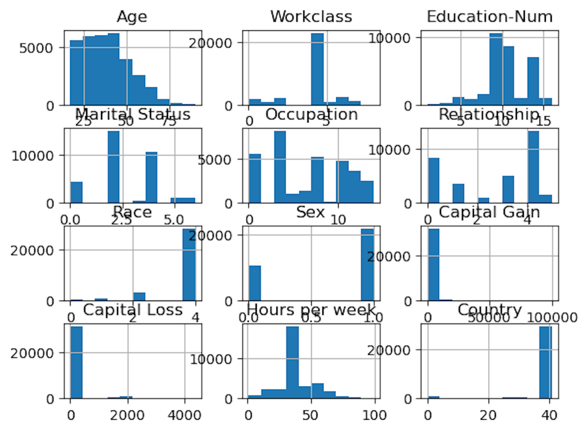
But as we can see it is not very well aligned and presentable.
- So, we have to add some parameters like bin, figsize and sharey. Let's discuss them one by one.
What is figsize in Histogram?
- Sets the size of the overall figure in inches.
- The figure size is specified as a tuple with width and height.
hist = X.hist(figsize=(10, 10))
- In this case, the width is set to 10 inches, and the height is set to 10 inches. But, still there is some space left in width, So, we can adjust accordingly.
- Let me try with 20 inch width.
hist = X.hist(figsize=(20, 10))
- This looks good. But, still I see bins are very less.
What is Bin In Histogram?
- Refers to an interval or range into which the data is divided.
- The data points are then counted or aggregated within each bin to create a visual representation of the distribution of the data.
- Default Value: 10
- I tried with multiple values, I found it, 30 seems to be gives a good histogram.
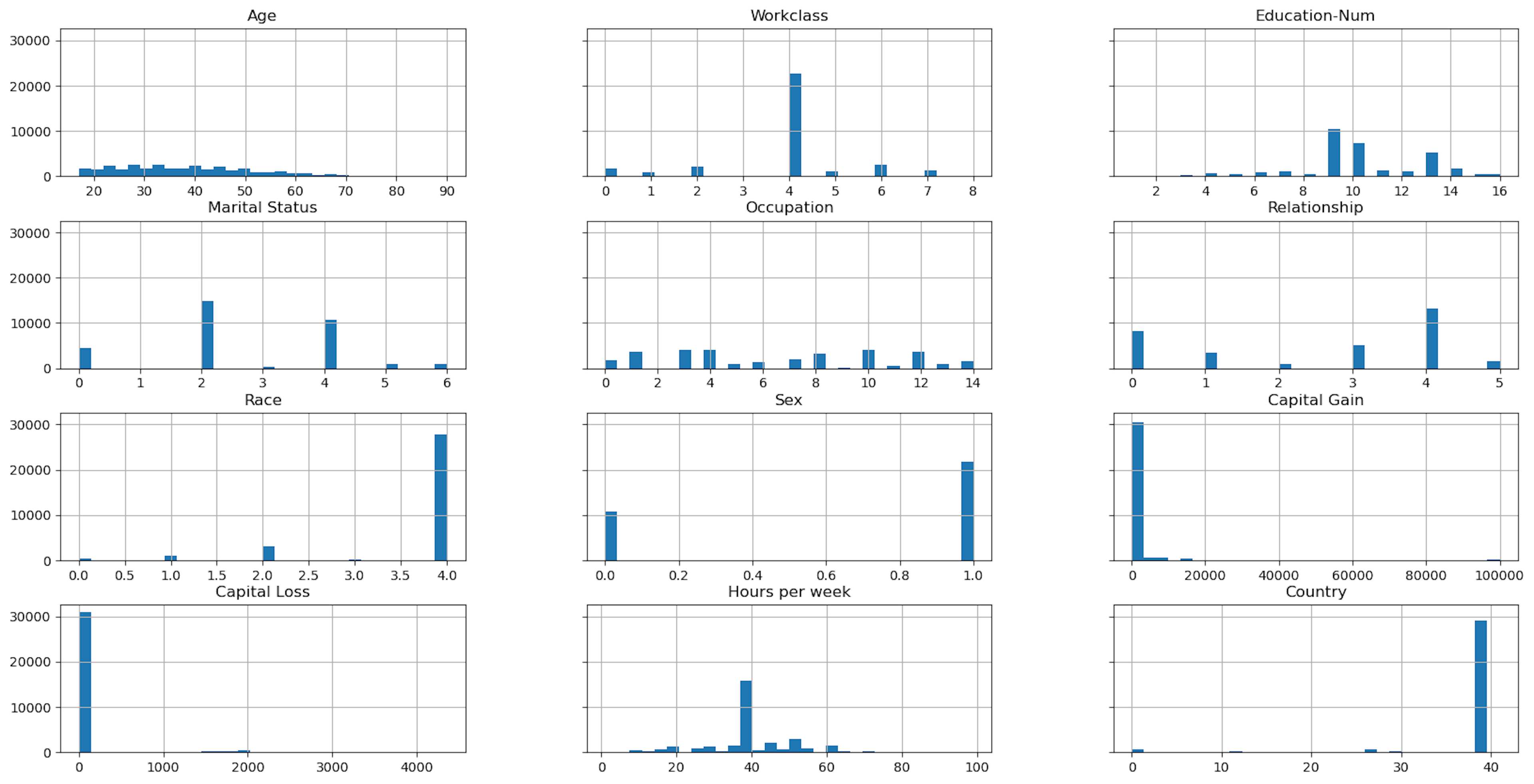
hist = X.hist(figsize=(20, 10), bins=30)
Output:
Important Note
- Choosing an appropriate number of bins is important in creating a meaningful and informative histogram.
- Too few bins may oversimplify the distribution, while too many bins may introduce noise and make it harder to identify patterns.
- The choice of bin size can impact the visual representation of the data, so it's often a good idea to experiment with different bin sizes to find the one that best reveals the underlying distribution.
What is sharey or sharex In Histogram?
- Specifies whether the y-axis or x-axis should be shared among histogram.
- When set to True, it means that all histograms will share the same y-axis or x-axis, making it easier to compare the distributions across different features.
- In our case, sharey=True will make our histogram more presentable, as main goal with histogram is correct and presentable representation of the distribution of data
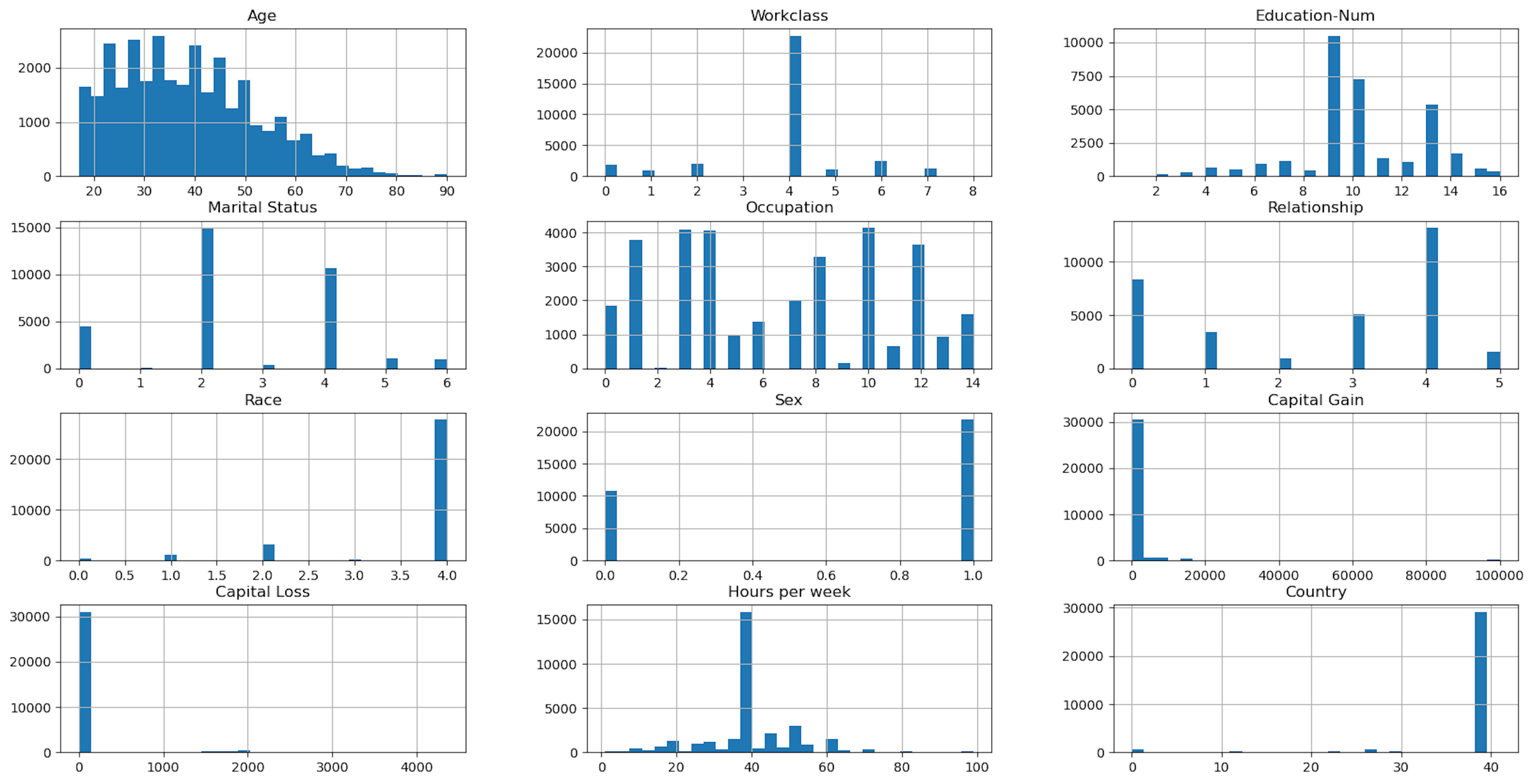
hist = X.hist(figsize=(20, 10), bins=30, sharey=True)
Output: